Data valuation for LLMs via Metagradients

Introduction

#

One of the most critical components of training a foundation model (e.g., an LLM) is the choice of the training data. A key challenge in designing the training data mix is estimating the value of different data,¹ and this often comes up in questions such as:

• What are the values of different data sources w.r.t. core model capabilities?
• Which new data source(s) caused a regression on the latest pre/post-training run?
• What was the counterfactual contribution of [some copyrighted work] on the model’s generations?

On one hand, answering these questions provides not only scientific value to the understanding of how data influences model behavior, but also enables researchers to efficiently ablate data mixes, providing significant savings in compute. On the other hand, these questions have implications beyond the model development—was Anthropic’s settlement with authors fair or should they have been compensated more? Is OpenAI paying too much or too little for its Reddit license?

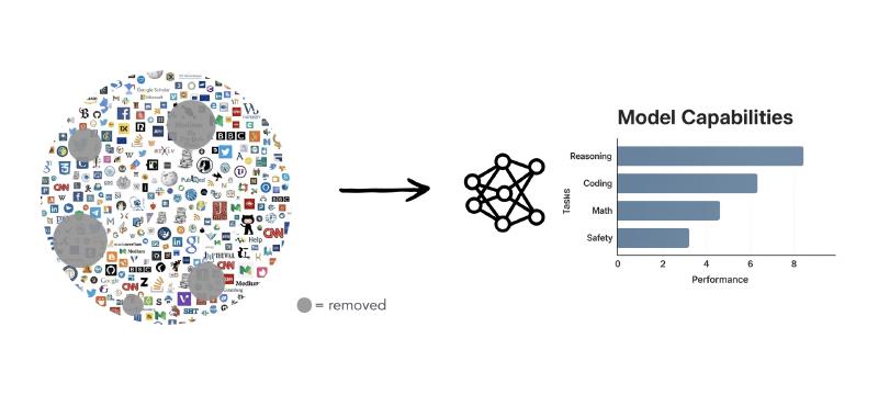
All of these questions reduce to a shared primitive—estimating how much the inclusion (or exclusion) of a subset of data influences the final model. While we do not tackle these applied questions directly in this post, we focus on developing and validating the underlying algorithmic machinery that would make answering them feasible.

While researchers routinely conduct coarse data ablations and general insights are known in the community (e.g., code contributes to general capability improvements beyond code [CTJ+21]), any analysis that is more fine-grained quickly becomes intractable. To illustrate: estimating the marginal (“leave-one-out”) contribution of 100 data sources would—without further approximations—require re-training 100 times in addition to the original run. As a result, one typically employs heuristics such as “micro-annealing,” but their fidelity remains unclear.

At a high level, there are two distinct challenges to developing efficient methods for data valuation:

1. Efficient algorithms: Designing algorithms themselves has been quite tricky historically (e.g., methods based on Hessian-based influence functions abound in the literature but did not reliably work at all until recently [GBA+23], [PGI+23]). On the flip side, it’s remarkable that an efficient approximation is possible at all!
2. Reliable evaluation: Even setting the question of estimation aside, evaluating algorithms is non-trivial due to the fact that the ground-truth is extremely noisy and expensive to compute.

We’ll see some evidence of the latter, but primarily focus on the algorithmic aspect of the former. Fortunately, there’s been a lot of amazing technical progress in the past few years and we now have algorithmic tools to approximate data values efficiently. In this post, we will look at how to formalize the data valuation problem, some high-level intuition for the two dominant approaches to this problem, and apply the recent metagradient approach [EIC+25] to pre-training (small) LLMs.

The data valuation problem

#

In plain terms, the data valuation problem asks: if we were to add or remove a particular data source from our training set, how much would the final model’s performance change [GZ19]? The challenge is that naively answering this requires re-training the model for every data source we want to evaluate, which is prohibitively expensive.

Let’s formalize the general problem as follows:

Consider some training corpus $\mathcal{D}$ (e.g., a text corpus scraped from the internet), some machine learning algorithm $\mathcal{A}$ (e.g., training a transformer with a specific set of hyperparameters) that maps a given dataset $S \subset \mathcal{D}$ to a trained model $\theta$, and some evaluation of interest $\ell$ that maps $\theta$ to a real value (e.g., eval on a benchmark).

The general goal of data valuation (or attribution) is to efficiently estimate $\ell(\mathcal{A}(S)) =: f(S)$ given $S$. That is, we want to predict the model outputs as a function of the training data alone [IPE+22]. Often, we (locally) approximate $f$ as a linear function and are interested in estimating the marginal or leave-one-out data value of a datapoint $i \in S$:

$$\nu_i := \mathbb{E}_\omega [f(S, \omega) - f(S \setminus \{i\}, \omega)],$$ where the expectation is over randomness $\omega$ of the training algorithm (e.g., weight initialization, data order, and GPU non-determinism).

In essence, this is a counterfactual estimation problem, and it is challenging as running an algorithm $\mathcal{A}$ in modern deep learning is extremely (computationally) expensive. How do we efficiently approximate such counterfactuals without re-training the model from scratch?

Note: while understanding the role of randomness is an important issue, we ignore it for the remainder of this post to focus on the fixed-seed setting, dropping the seed term $\omega$ as it remains fixed. In practice, this is achieved by using the same initialization, which naturally subsumes cases like continued pre-training or fine-tuning (which begins from some fixed checkpoint), provided the data order remains fixed.

Background: a tale of two algorithms

#

A long line of work on influence function approximation (originating from robust statistics [HRR+86], [P81], and introduced to machine learning by [KL17]) followed by more recent machine learning research on data attribution [HL22] aim to develop efficient and reliable approximations of $f$ (typically by estimating the marginal data values $\nu_i$).

Despite the incredible variety of approaches, they all essentially aim to replace the above re-sampling estimator with its local approximation. To do this, we generalize the definition of $f$ (and our learning algorithm) to operate over continuous weights, e.g. $f$ now takes input in $\mathbb{R}^{|\mathcal{D}|}$.

Then, we approximate the marginal data value relative to train set $S$ as the derivative: $$ \nu_i \approx \lim_{\epsilon \rightarrow 0} \frac{f(\mathbb{1}_S + \epsilon e_i) - f(\mathbb{1}_S)}{\epsilon} $$ where we upweight the i-th example by $\epsilon$ and $e_i$ denotes the i-th basis vector.

At a high level, there are two kinds of approaches to approximate the above derivative: we’ll refer to these as “implicit” vs “explicit” differentiation methods.

Implicit differentiation methods (the most prominent being the influence function) characterize the final model as a local minimum to an empirical risk minimization problem, and use a Taylor approximation to estimate how perturbing the data weights affects this minimum. Notably, these methods typically only probe the final checkpoint and do not require re-training or knowing how we got to the optimum.

Explicit differentiation methods, on the other hand, consider the entire trajectory of iterative optimization (e.g., the iterates taken by SGD or Adam), and explicitly differentiate through the entire computational trajectory to compute the exact gradient, i.e.,

$$ \nu_i \approx \left. \frac{\partial f(w)}{\partial w_i} \right|_{w = \mathbb{1}_S} $$

The key insight is that typically in modern deep learning, the entire sequence of operations taken by $\mathcal{A}$ is—however complex—some differentiable function of the data weights $w$, so one can “just differentiate” through the entire learning algorithm using standard autograd libraries. Computing this derivative can be extremely expensive if one’s not careful, but the object is nonetheless faithful to the actual optimization trajectory.

These methods have a long history in meta learning, hyperparameter optimization, and even fields like PDEs (where it is better known as the “adjoint” method; e.g., to analyze the sensitivity of a PDE to initial conditions). More recently, the metagradient method [EIC+25] takes this approach and—with some clever insights and implementation—demonstrates its effectiveness across various large scale models and even settings beyond data attribution.

In the rest of this post, we will apply the metagradient approach to language model training to tackle the problem of approximating marginal data values.

Smoothness: when are metagradients well defined?

#

If we can differentiate through everything, isn’t the influence estimation problem solved? Not quite—the metagradient is an extremely ill-behaved object in general. In fact, for standard settings, if you compute it, you will just get NaNs due to gradients blowing up.

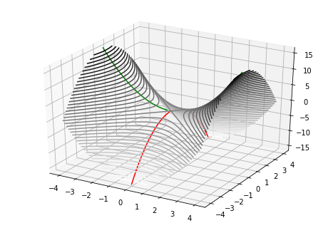
One intuitive way to see why this is the case is as follows: suppose during training the current iterate is at a saddle point, and there are two potential “basins” A and B the trajectory can converge to. An infinitesimally small perturbation can determine whether the optimization descends into A or B—basins that are a finite distance apart in parameter space. The derivative is thus effectively infinite.² So if you imagine that earlier in training, the optimization is exploring many potential “basins”, it’s no surprise that metagradient is infinite w.r.t. that trajectory (and many alternative ones).

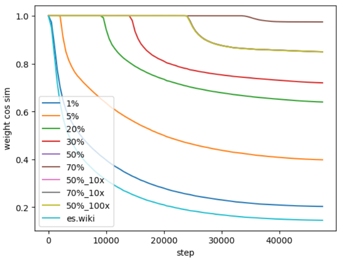
Indeed, one can see that a single data perturbation early in training can cause the trajectory of weights to completely diverge. In the experiment below, we examine the sensitivity of pre-training a GPT-2 model with a fixed data order. Across different runs, we introduce a perturbation by zeroing out the gradient of a single example in a batch at different points in time, tracking the evolution of the cosine similarity of one of the weight matrices throughout training. Notably, any perturbation before halfway into training causes significant divergence in weight space (< 0.7 cosine similarity). ³

So when do we expect metagradients to be useful? Intuitively, we want the local landscape to look approximately linear in the data perturbations. [EIC+25] characterize this intuition more rigorously using a metric called metasmoothness. While the metasmoothness is very low for standard training hyperparameters and architectures, the authors find that in many standard settings you can tweak hyperparameters a little bit to find configurations that have much higher smoothness. (However, this gain typically comes at a small cost in loss, and it is an open question to understand the exact tradeoffs between smoothness and loss.)

Metagradients for pre-training

#

We focus on pre-training as it is arguably the most interesting setting to study this algorithm:

• Because modern pre-training operates in a heavily undertrained regime (~one epoch over the data), it clearly departs from the assumptions of the implicit differentiation approach (which assumes a well-converged local minimum) and demands using the precision of an explicit approach.
• Pre-training takes much longer than fine-tuning and is a good testbed to test the limits of metagradients over extremely long horizons, and has not been studied in prior work.
• Pre-training consumes by far the most amount of raw data; hence, understanding the value of data is particularly important for i) optimizing pre-training data mix, but also ii) giving us a tool to precisely quantify the value of data (e.g., for data pricing, as we motivated in the introduction).

Now that we’ve laid the conceptual groundwork, we can now look at applying metagradients to LLM (pre)training.

Results

#

We first look at pre-training (training from scratch) a modified GPT-2 style transformer.

Pre-training

#

Setup. We train a 124M parameter transformer⁴ on 1.6B tokens of text data sampled from RedPajamaV2 [W+24]. Since the training corpus consists of a vast number of domains, we isolate the top 20 domains by token count and estimate their data values.⁵ In particular, we approximate the value of a domain as the sum of the values of its constituent documents seen during training. As a target metric for data values, we use the LAMBADA task, a standard benchmark for long range understanding.

We compute both an estimate of the ground-truth data value by re-training models on the corresponding counterfactual training sets (i.e., after removing the $i$-th data source) as well as our approximation to it based on the metagradient (computed using an implementation of REPLAY [EIC+25]).

$$ \text{(ground-truth)}\;\; \nu_i = f(S) - f(S \setminus \{i\}) $$ $$ \text{(metagradient approx.)}\;\; \nu_i \approx \frac{\partial f(w)}{\partial w_i} $$

To keep our analysis in the metasmooth regime, we hold fixed the first 8% of training (using identical data and data ordering across all runs) and compute counterfactuals and metagradients only over the remaining 92%.⁶

Remark: we hypothesize that marginal data differences only manifest past the initial phase of training, as early in training the learning dynamics focus more on, e.g., memorizing frequent n-grams [CTB23], but this remains to be verified.

Findings. As the domains vary substantially in their size, we analyze their token normalized data values (i.e., adjusted by their relative token count). We find that we can approximate ground-truth data values accurately (rank correlations of $r \approx 0.85$); see Figure 4. While re-training the model separately for each of hundreds or thousands of domains would be computationally infeasible, using metagradietns allows one to estimate many such counterfactuals simultaneously using only $\sim$3x the compute of the original model training. In fact, while we aggregate and perform analysis at the level of individual domains, we obtain estimates for marginal data values at the document level, which would be completely infeasible using re-training!

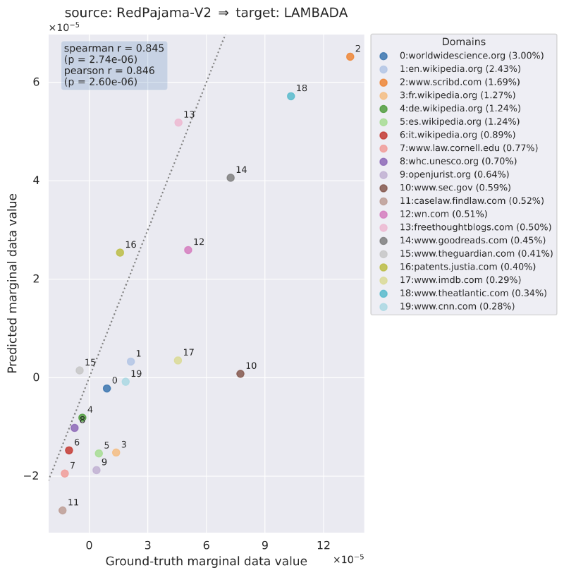
Among the top domains analyzed, scribd, theatlantic, and goodreads have the largest relative data values. In a separate analysis, we found that some less common domains such as aparchive (not shown in Figure) have remarkably higher normalized data values than these top domains, suggesting that future data curation may benefit from a more fine-grained analysis of each domain’s contribution that goes beyond simple heuristics such as size or human-engineered notions of data quality.

Smoothness interventions on hyperparameters and architecture. Building on the findings of [EIC+25], we confirm that specific hyperparameter choices—such as using smaller learning rates, adding a small $\epsilon$ inside the square root of the Adam update denominator, using lower LayerNorm $\epsilon$ values, and tuning parameter initialization (e.g., no bias parameters and $\mu$P)—significantly improve metasmoothness.

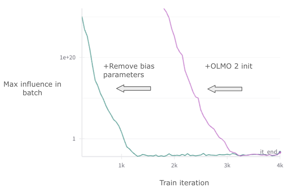
Furthermore, we find that modern, standard architectural components like RMSNorm and Rotary Position Embeddings (RoPE) also help improve metasmoothness.

Science of data valuation. Our investigations thus far confirm two challenges to (statistically) meaningful data valuation: First, training is a stochastic process, and the ground-truth estimates can vary significantly between different runs, making it challenging and computationally expensive to assess the validity of any single estimate. Second, even the true influence function (as computed by the metagradient) is often unstable, particularly near the beginning of training; intuitively, as discussed earlier, this is because early in training any small perturbation can still cause the training to diverge to very different final “basins” of the loss. One valuable direction for future work would be a general analysis and prescription of when and how reliable attribution can be achieved given these factors.

Continued pre-training

#

To complement the above results on pre-training and to replicate similar results from the original paper, we now investigate continued pre-training (which one could view as a fine-tuning regime).

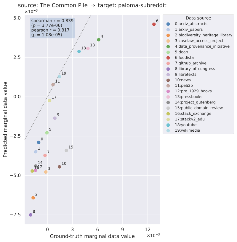
Setup. We take a pre-trained 124M model (same architecture), this time already fine-tuned on 3.2B tokens of text data from FineWebEdu. Subsequently, we fine-tune this model on 20 uniformly weighted data sources from the Common Pile corpus. We then evaluate the fine-tuned model on Paloma-subreddits, a standard perplexity evaluation benchmark based on a collection of reddit posts; one may view this as a proxy for the model’s understanding of informal, user-generated web discourse.

Findings. Similar to pre-training, we find that metagradient-based approximations yield reasonable approximations to true marginal data value of data sources.

Approximations to metagradients

#

One natural question is to what extent it’s necessary to compute the “full” metagradient. Is it possible that we can approximate it by only looking at, for example, “suffix” or tail end of the trajectory? (This would also lend more credibility to the usual heuristic of using “microannealing” or “tail patching”.) Unfortunately, the following analysis indicates that this is not the case:

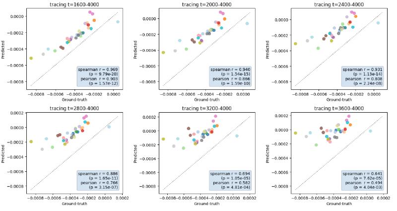
In this experiment, we took the partial sums of the metagradient scores (recall that we have this for every document / example) corresponding to different suffixes of training. Specifically, we approximate the marginal value of a data source by summing up the metagradient estimates for all the documents belonging to a particular suffix of the trajectory. We can observe that the predictability degrades quickly as the included trajectory gets shorter. This result suggests that any naive attempt to “cheat” by observing only partial trajectory will likely fail.

Conclusion and future work

#

These results demonstrate that fine-grained approximations to data values in pre-training can be tractable and effective. Prior work focuses mostly on large data counterfactuals (e.g., less than ten data sources analyzed) or on a different regime of training (mostly fine-tuning). One exception is TrackStar [CRB+24], which shows that using a well designed implicit differentiation method can scale to pre-training; however, it focuses on attributing individual model outputs rather than aggregate metrics.

To conclude, we share some thoughts on directions for future work:

• Stronger baselines and new algorithms. Better understanding the effectiveness (and failure modes) of baselines such as micro-annealing would be practically extremely valuable. Algorithmically, we are perhaps just getting started as it is only in the past few years that we first have scalable, predictive methods.
  • The two (and perhaps the only effective) algorithms are based on implicit and explicit differentiation. Is there a way to combine the benefits of both approaches to yield a stronger algorithm? There is some really nice initial work in this direction, e.g., [BLL+24].
  • Developing better algorithms will also require a deeper understanding of the nature of randomness and learning dynamics of neural networks and how they interact with marginal data values. (E.g., as we remarked before, earlier in training might be extremely unsmooth in terms of optimization dynamics but perhaps inconsequential for purposes of data valuation when marginalized over randomness.)
• Scaling of data values. It is common practice to perform data ablations at a much smaller scale and then extrapolate to the relevant scale. What are the right adjustments and functional forms needed to extrapolate accurately?
  • If it turns out there are accurate scaling laws, we might be able to do away with simpler (but more expensive) approaches like regression done at smaller scale (e.g., using tiny swarm-based models in Olmix [CMH+25]) rather than using influence approximations (which can be done at larger scale but are more sensitive to hyperparameters).
  • There is some nice initial work in this direction, e.g., [CJH+24] and [OGK+25], though the former only looks at the scaling along data scale (whereas we need to look at scaling in both model size and data) while the latter is based on the premise that micro-annealing is a good approximation to the true counterfactuals.
• Science of data quality. What approaches like metagradient make feasible for the first time is (efficiently) performing “thousands of ablations at once”. With this data now available (or easy to compute), further analysis can guide practitioners (e.g., those looking to acquire data to improve models), data creators (e.g., those looking to get compensated for their data), and policy makers (e.g., determining the significance of data sources in the context of copyrights). Alternatively, the data from these hypothetical ablations may be used to train better cheap fast data quality estimators (e.g., fasttext classifiers as used in DCLM).
• Beyond linear estimators. Almost all work in this area is based on local linear approximations to data. An important open question is understanding—both theoretically and empirically—when non-linear effects manifest and how to predict them (e.g., when two data sources are individually helpful but together detrimental).
  • One common way to deal with the non-linearity is to iteratively compute metagradient and run gradient descent in “data weight space” [EIC+25]. While simple and elegant, this approach is extremely expensive, and we suspect there are other ways to correct for the non-linearity.
• Data valuation for RL. A significant component of the modern LLM pipeline is RL during post-training. Extending existing approaches for data valuation to this regime is tricky, however, as the data (e.g., the model’s attempted solution) is generated online by the model itself. We think that a lot of creative approaches are possible here.

Code

#

Coming soon!

Acknowledgements

#

SP would like to thank the Stanford HAI Hoffman-Yee grant for funding his postdoc, the Stanford Marin team for the infra support (special thanks to David Hall, Ahmed Ahmed, and Suhas Kotha), Google TRC and Stanford NLP for generous compute, Andrew Ilyas and Logan Engstrom for an initial codebase for metagradients to jump start the project as well as various tips and discussions, Tristan Thrush for helping with initial pre-training code and data, Marcel Rod and Tatsu Hashimoto for an elegant re-implementation of metagradients, Sally Zhu for some analyses and experiments on metagradients (not discussed here), Yu Sun and his team for discussions on meta-optimization, and finally various members of p-lambda, Hashimoto lab, and Zou lab for useful discussions.